Tools for Visualization and Analysis of 4D Shapes in SlicerSALT

We have recently published our SlicerSALT 5.0 release. One of the main updates to SlicerSALT is the addition of tools and functionalities for the visualization and analysis of 4D shapes that are composed of sequences of 3D geometries.

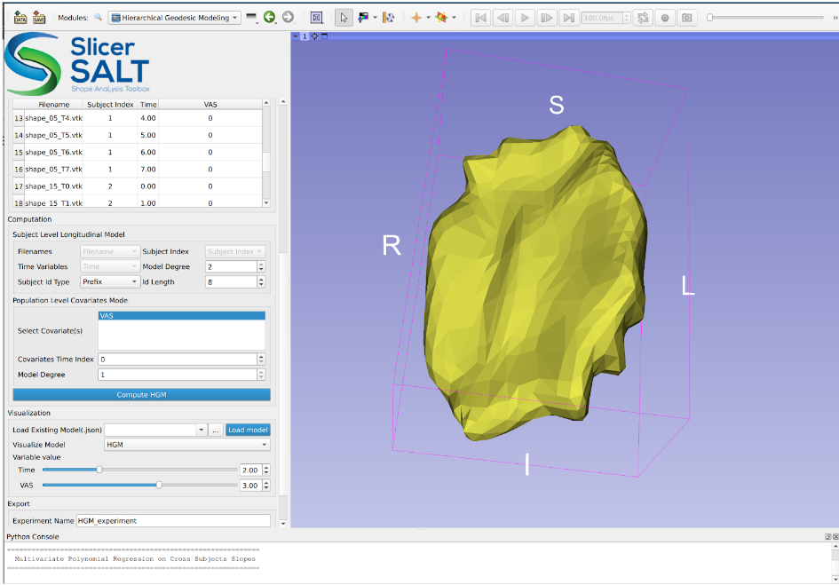
As part of this release, we have created a new module named Hierarchical Geodesic Modeling that is designed for the computation, visualization, and analysis of longitudinal shape models using geodesic-based shape modeling methodology. 

Once correspondence has been established within a population of shapes (point distribution models), this module can compute (i) continuous trajectories of the shape change of individual subjects, over a common continuous variable (i.e. time), (ii) a mean trajectory of all input subjects and (iii) a hierarchical geodesic model (HGM) based on selected covariates that enable our users to relate structural changes over a continuous variable with function. The exported modeling result from this module can be paired with updated functionality in Shape Population Viewer to allow multi-subject visualization of 4D shapes. Here, we present a brief introduction on how to use the Hierarchical Geodesic Modeling module to analyze 4D shapes and visualize/record the computation results.

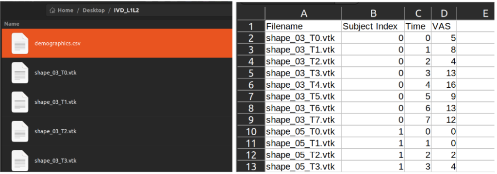
Two inputs are required for using this module:

1. An input directory that contains all the correspondent shape files in “.vtk” format.
2. A demographics(.csv) file that has the information for each shape file including filenames, subject index, time variables and covariates.

After the user clicks the “Load Data” button, the loaded data will populate the module table and preload the option/parameter entries.

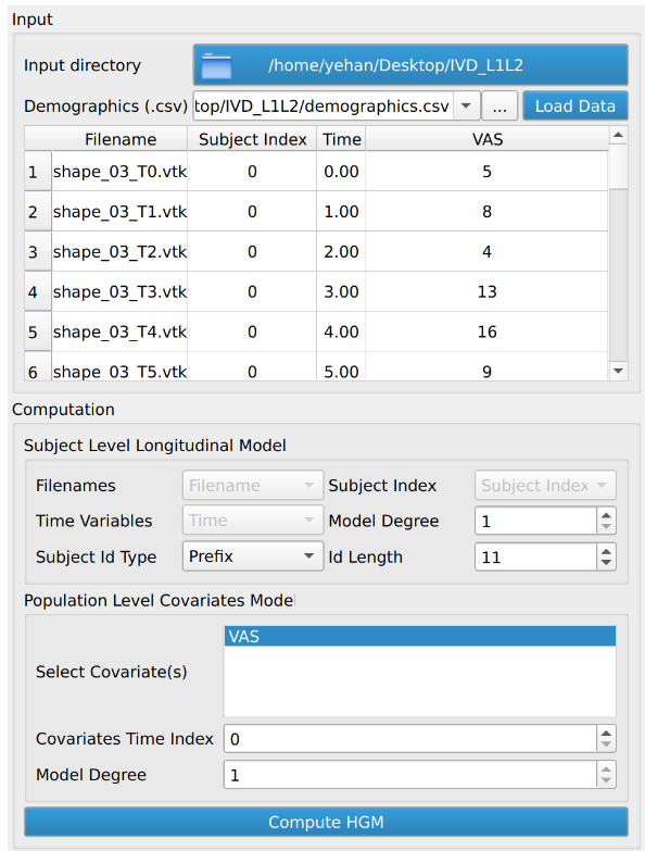
A user needs to decide two sets of parameters/options, namely the subject level longitudinal model and the population level covariates model. For the subject level model, the user needs to set the degree of the individual subject’s longitudinal geodesic polynomial model and the subject id for visualization and export. For the population level model, the user needs to set the choice of covariate(s) for computing HGM and the degree of the population level covariates model. A higher degree generally means a tight fit to the longitudinal observations at subject level or to the regressed individual level parameters at population level.

After confirming the options/parameters, the user may click the “Compute HGM” button to fit geodesic models to the input shapes. Three types of geodesic models (mean, HGM and subject trajectories) will be generated and can be visualized using the module’s interactive sliders in the visualization section. Subject trajectories are the geodesic polynomial models representing the continuous trajectory of the shape change over time of individual subjects. Mean trajectory is the geodesic polynomial model obtained by averaging fitted model parameters from all individual subjects. The mean time 0 point is the Fréchet mean of all subjects’ time 0 points. The tangent vectors (model parameters) are the mean tangent vectors of all post-parallel-translation tangent vectors of all subjects. The HGM trajectory is the hierarchical geodesic model as described in our IPMI paper, which can show how shape changes with respect to both the time variable and selected covariate(s).

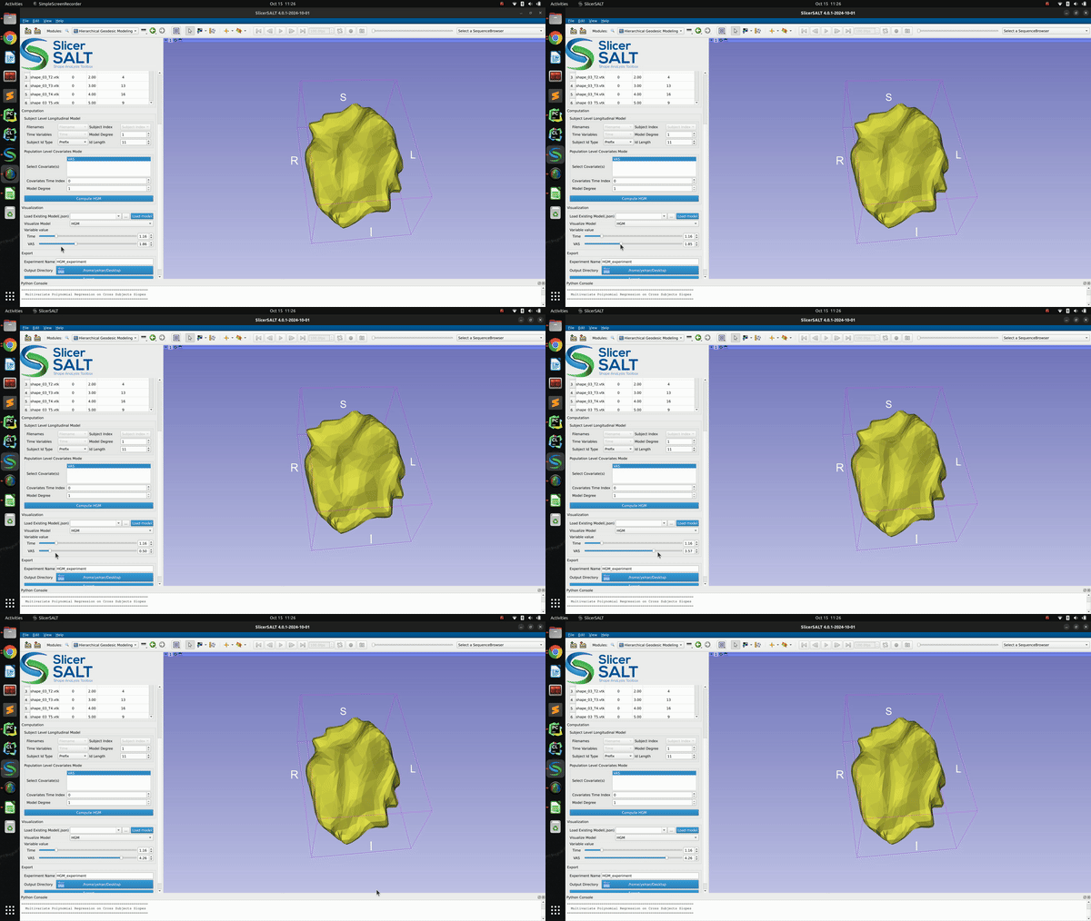
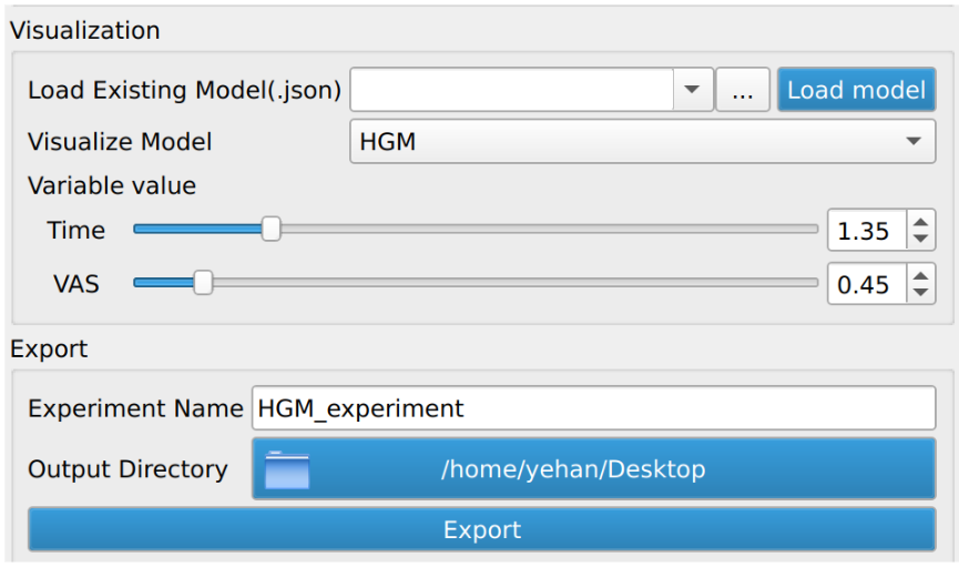
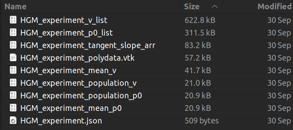
The successfully computed results can be exported to a user selected directory as a metadata “.json” file, a reference polydata and all the geodesic model parameter files as shown in figure below. The saved computation results can be reloaded to the module by selecting the exported “.json” file and clicking the “Load model” button.

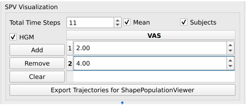
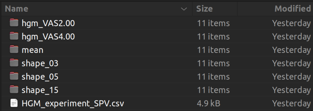
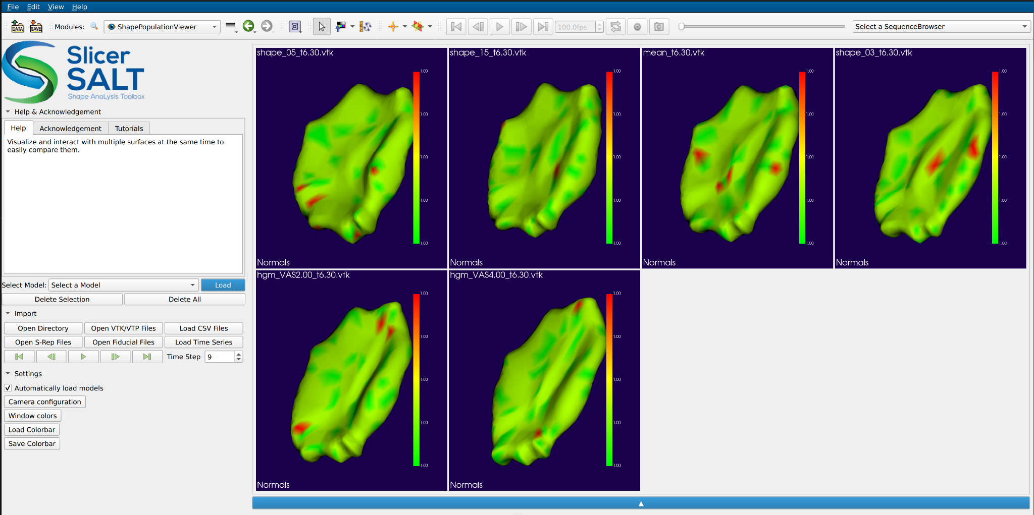
In addition to the model export, we also added functionality to support time series visualization in SPV. Users may check “Mean”, “Subjects”, and/or “HGM” to export trajectories of interest to the selected output directory. These trajectories can be then visualized in SPV by clicking “Load Time Series” and selecting trajectories (rows) of interest from the exported “.csv” file.

Additional notes:

• Input shapes (point distribution models) need to be in correspondence. This can be achieved by generating a template model and using the mesh-to-mesh tools available in SlicerSALT to propagate the topology throughout the input shape population.
• Although we use the notion of “time variables” in demographics, it can be any continuous independent variable of interest users want to regress against at the subject-wise level.
• Visualizations for varying covariates at the same time point in SPV can be created by only exporting the HGM trajectories, transposing the exported .csv file and loading it from the SPV.

For more information, please see the module’s github page. We encourage users to provide feedback and ask questions by creating github issues.

SlicerSALT is made possible through contributions from a multidisciplinary team coming from Kitware, NYU Tandon School of Engineering and The University of North Carolina at Chapel Hill. The development of SlicerSALT is supported by the NIH National Institute of Biomedical Imaging Bioengineering R01EB021391 (Shape Analysis Toolbox for Medical Image Computing Projects).

SlicerSALT is an example of custom 3DSlicer applications that Kitware develops. Contact us at kitware@kitware.com to learn how we can help you integrate the 3DSlicer-based software into your research, processes and products.