Following a recent CC-FR webinar High fidelity simulations with OpenRadioss™ & ParaView by Altair and Kitware, this blog post describes an example of workflow to post-process OpenRadioss results with ParaView. OpenRadioss is a free, publicly available FEA software for simulation of impact, shock and highly dynamic events, actively developed by Altair. 

The example data is a cell phone drop simulation that you can download from the OpenRadioss website, and run on your personal computer following the instructions. The simulation generates ‘anim’ files, ending with AXXX, and a time history file, ending with T01.

Open the anim files in ParaView: vtk, vtu and VTKHDF

The first step is to open the data in ParaView. Currently, there is no dedicated reader for the anim or the h3d file format, so you must convert your result to a ParaView compatible file format.

OpenRadioss provides a simple tool named `anim2vtk` which produces VTK simple legacy format, ASCII variant. This file format is easy to write, but very slow to read in ParaView. We recommend converting your vtk files to vtu file format to achieve significant performance gain. To do so, you open the VTK file in ParaView then use “Menu->Save Data” and select the vtu file format in the dialog box. You can open the VTK Legacy format as file-series to convert several time steps at a time.

However, a more efficient approach is to convert anim files to VTKHDF file format by using the dedicated tool openradioss-to-vtkhdf developed by Kitware. The advantage of using VTKHDF is read performance, automatic parts extraction with names and having only one file for all the time steps, which also allows writing the cell types and connectivity only once. Below are some size and performance comparison charts between anim, vtk, vtu and VTKHDF data formats, where lower values are better:

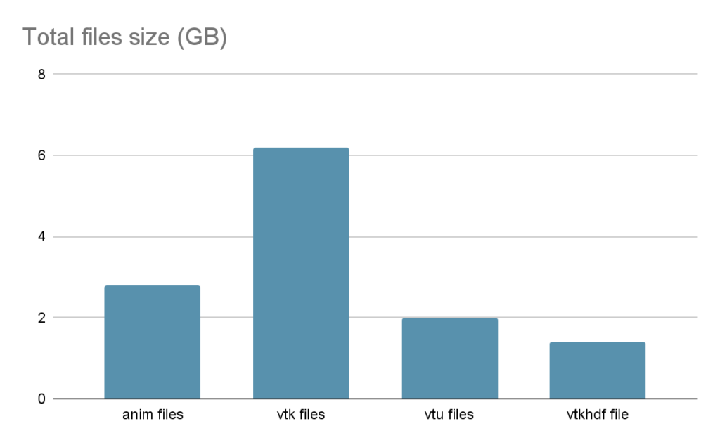
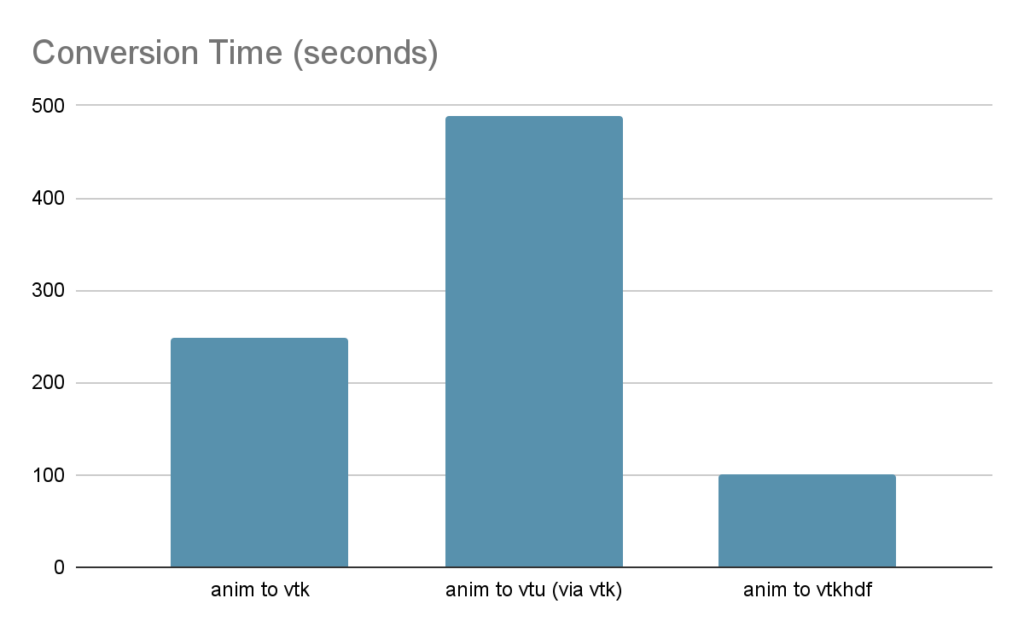
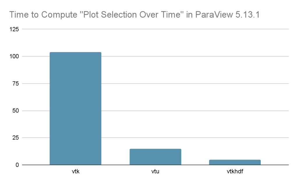
In a nutshell, you should use the VTKHDF file format to efficiently post-process your data in ParaView.

Display Geometry, Mesh and Parts

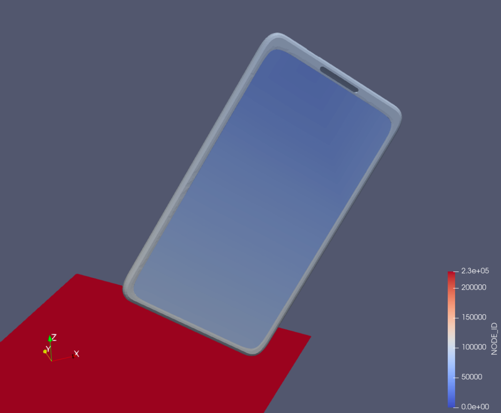
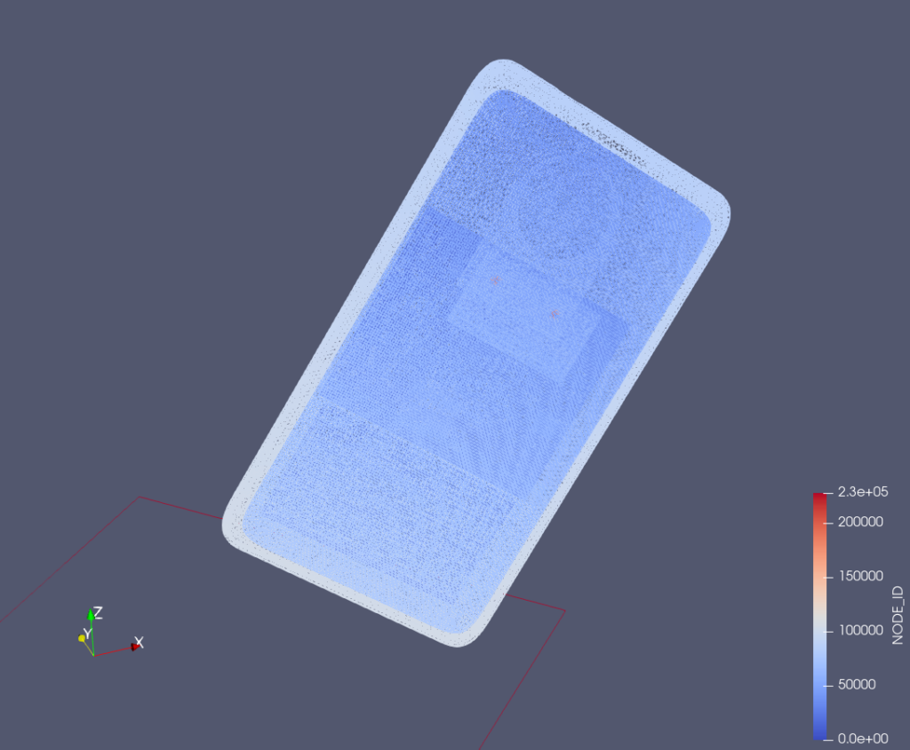
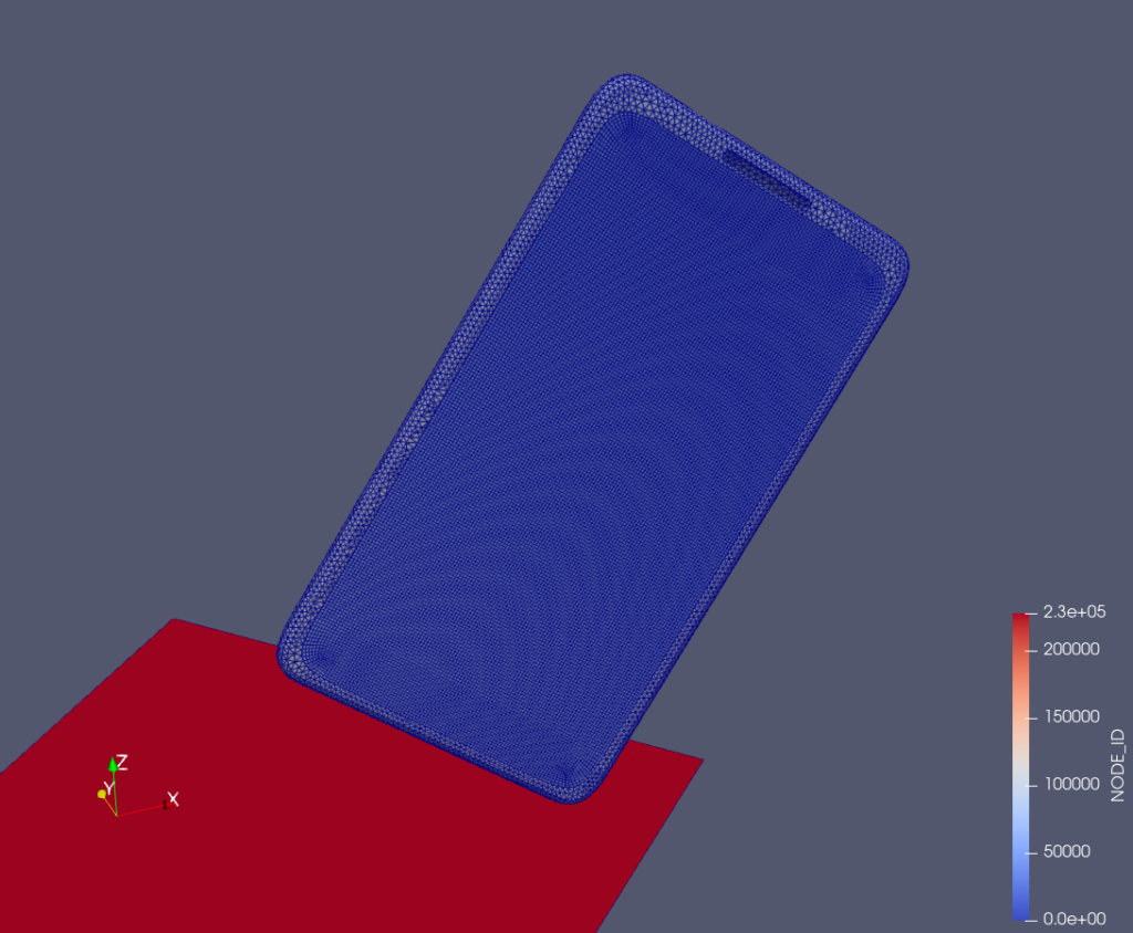
After converting the data and opening the file(s) in ParaView, the first step is usually to check the geometry and mesh of the model. ParaView offers a variety of representations and display parameters that we can combine:

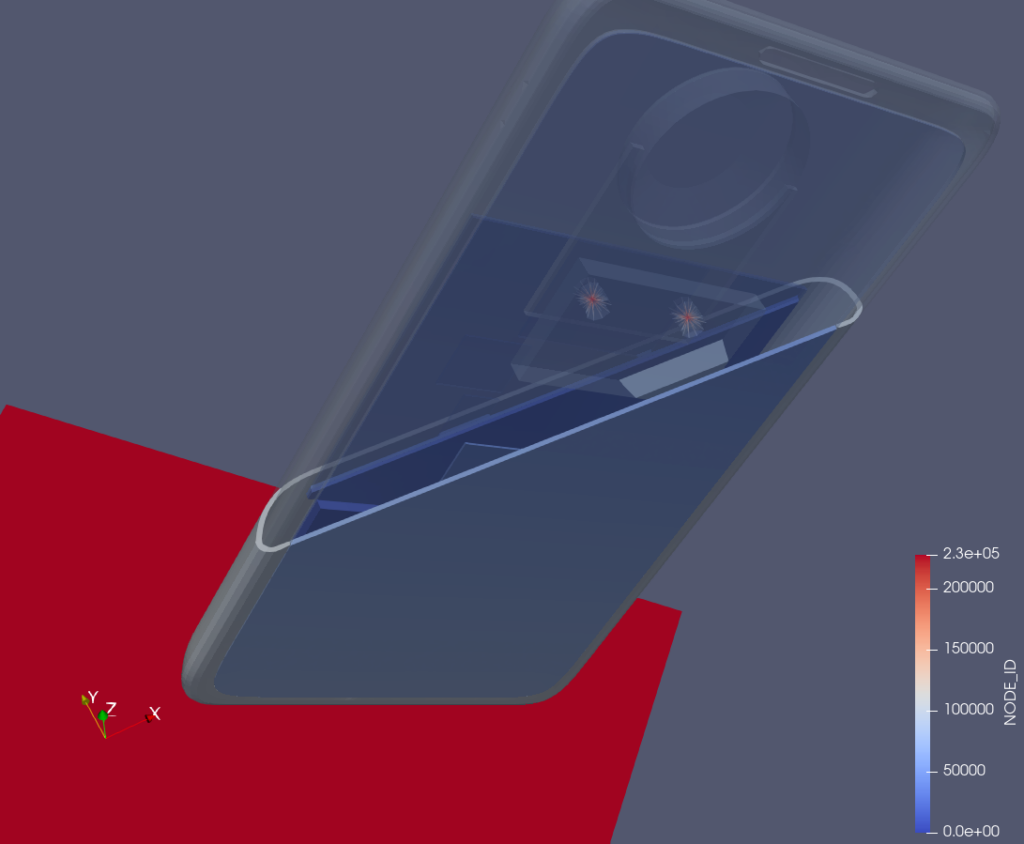
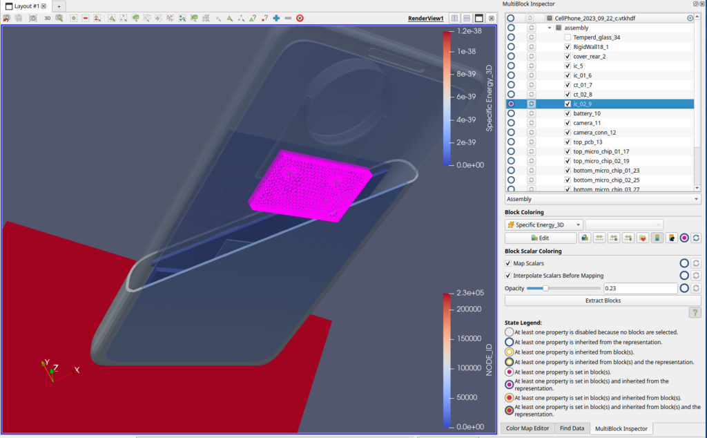
If you are using the VTKHDF file format, you can use the multi-block inspector to select, highlight, hide any part, and apply separate block coloring:

Display Stress and Deformation

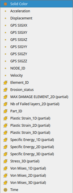
Then we need to check the simulation results such as Stress and Deformation. You just have to select the desired field in the combo box, then the coloring and the legend should adapt accordingly.

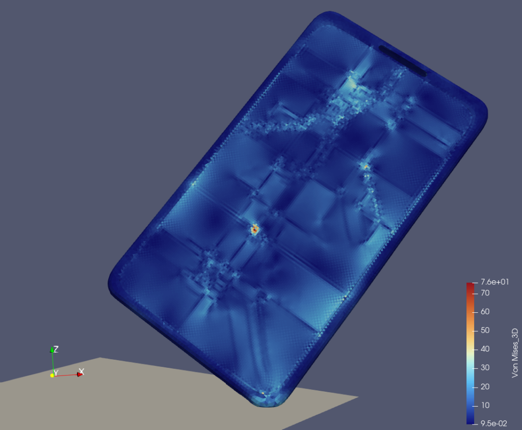
You can play time with the upper toolbar, and get the evolution of the Stress or Strain or criteria for each time step.

Plot Eroded Cells Over Time

One interesting post-processing technique for shock analysis is to measure the evolution of the cracks over time. As demonstrated in the previous paragraph, we can see the eroded cells on the glass, but where are these cells and how many cells are eroded over time?

To answer this question, we’ll use the Find Data Panel which you can enable via the View menu. The Find Data feature is a very powerful tool to select points or cells based on queries like “select all points with ID between 100 and 200, and stress magnitude greater than 0.5”. More information in the Selecting Data ParaView documentation.

In our case, we just have to choose the data producer, the element type and the query “Erosion_status is 0”. After clicking “Find Data”, the eroded cells are selected in the 3D View:

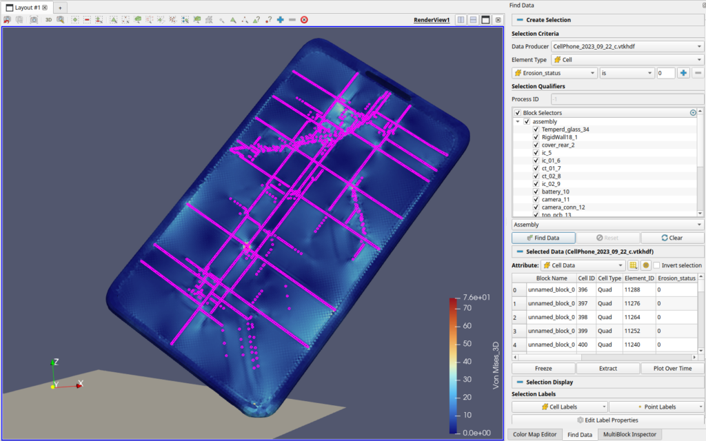
You may then click “Extract” to generate a dedicated dataset with only the eroded cells, and also click “Plot Over Time” to plot the evolution of the extracted data over time:

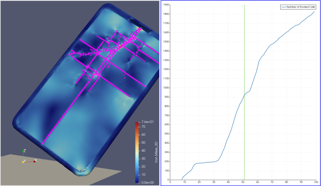
As you’ve extracted the eroded cells, you may want to display them in a dedicated color, thanks to the pipeline browser and the Color Map Editor:

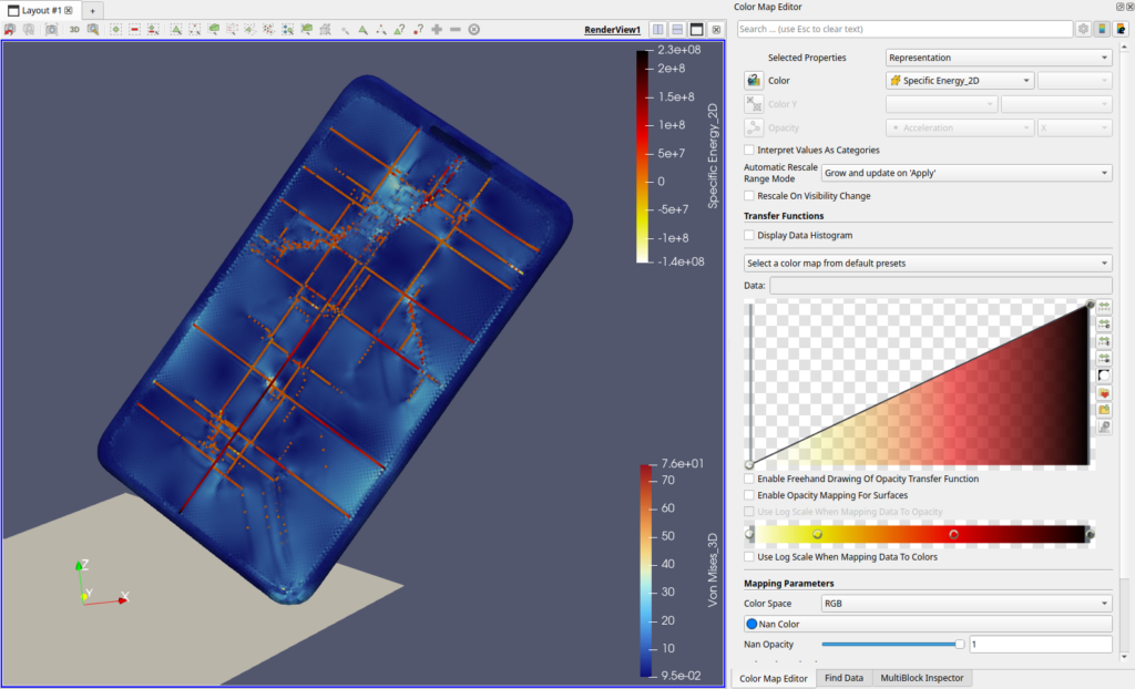
To go further with the crack propagation, you may look at the Topology Toolkit Plugin in order to detect the network topology and compute metrics.

Display Time History Values and Derivatives

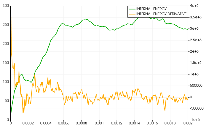
OpenRadioss simulation also generates a T01 file, which contains global variables evolution over time, such as Contact Energy or Momentum. After using the OpenRadioss built-in tool `th_to_csv` you can open the generated csv file in ParaView and plot the values over time by creating a line chart view:

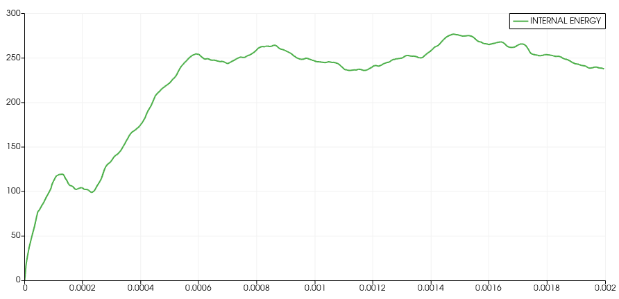
A popular analysis is to compute derivatives of some of the values. Using the current csv file structure there is no direct way to do it, but the python capabilities of ParaView come to the rescue!

Let’s create a Python Calculator, activate the multi-line expression, loop over the time steps and do the finite difference computation. The code to compute the derivative of Internal Energy is displayed below : 

import numpy
from paraview.vtk.util import numpy_support

valueArray=numpy_support.vtk_to_numpy(inputs[0].RowData['INTERNAL ENERGY'])
timeArray=numpy_support.vtk_to_numpy(inputs[0].RowData['time'])

outputArray2= numpy.diff(valueArray)/numpy.diff(timeArray)

return np.insert(outputArray2,0,0)

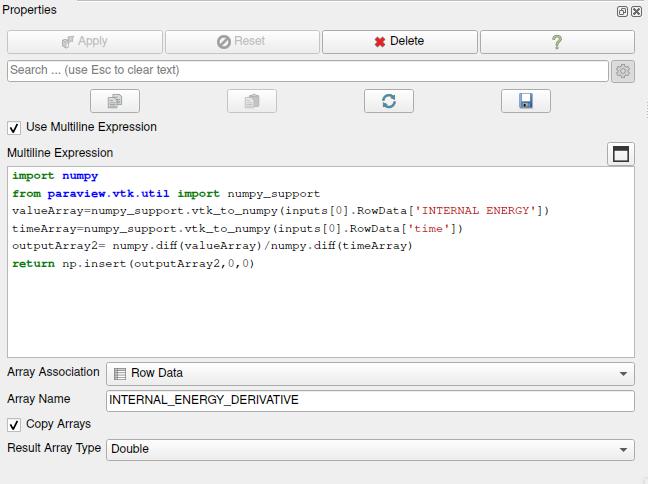
Then you can display this new curve in the same line chart as the internal energy:

Realistic Rendering

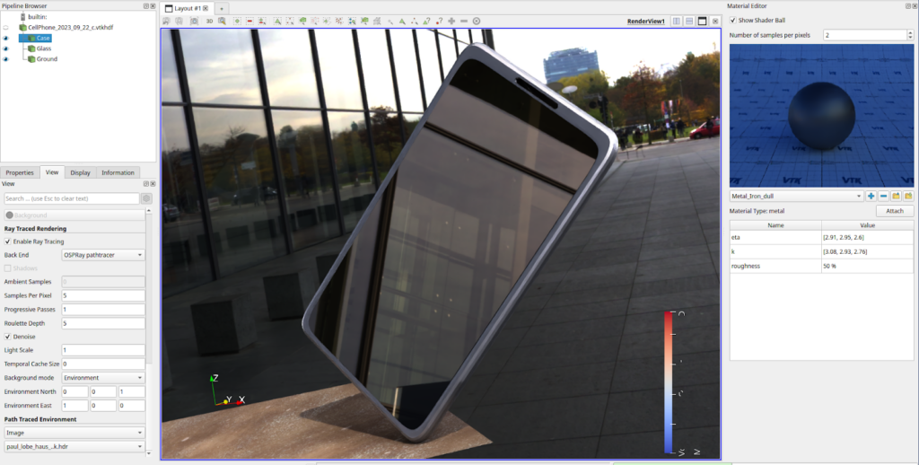
ParaView offers lots of advanced post-processing features. For example, you may want to leverage realistic rendering by using Ray Tracing back-ends like Intel OSPRay or NVidia OptiX. 

The usual workflow is to extract the parts you want to display with advanced rendering, then apply material and trigger the ray tracing rendering. In our case, let’s extract the ground (block ‘RigidWall18_1’), the case (block ‘cover_rear_2’) and the glass (‘Temperd_glass_34’).

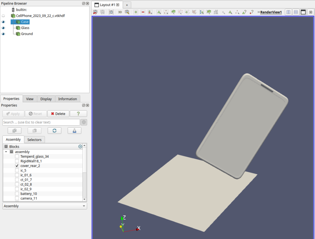
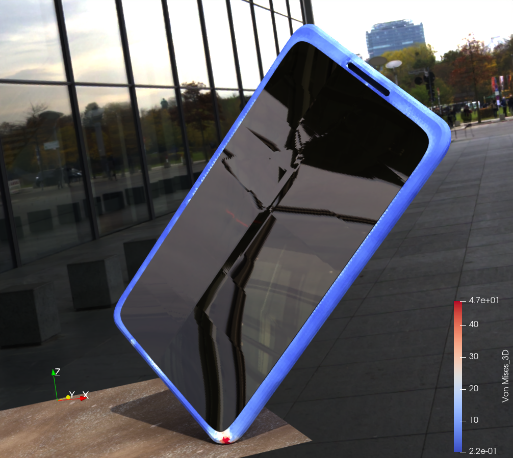
Then, let’s activate the ray traced rendering in the properties and open the Material Editor with the Shader Ball. We’ll apply a material to each of our parts: PBR_Ground_Dirt for the ground, Metal_Iron_Dull for the case and Metal_Copper_mirror for the glass. Next step is to add a skybox to get environment lighting and tweak the light to get realistic rendering:

Of course you can combine data coloring with advanced rendering by removing the material of the case and choosing the Von Mise criteria instead:

The full workflow is detailed in the Advanced rendering of scientific data using ray-tracing in ParaView Webinar and in the ParaView Material Editor blog.

Advanced Post-Processing

The ecosystem around ParaView is very rich, and you can manipulate your data through a large number of media and devices very easily. A typical example is the immersive plugin, which lets you visualize your data in Virtual Reality and Advanced Reality headsets like Oculus Rift or Microsoft Hololens:

More information in the Navigation Basics in Virtual Reality with ParaView blog post.

In addition, thanks to the python API, you may also plug any python library like PyTorch in order to run AI inference in ParaView. This is very useful to explore surrogate models based on dimension reduction or Deep-learning techniques. You can even view inference results and monitor the training process in real time with ParaView Catalyst!

To easily share your data with your colleagues, you may also export to Kitware Glance, in order to get a light web app to explore your dataset in 3D. Just select File->Export Scene… then choose VTKJS file format.

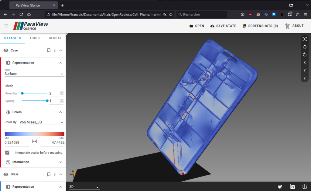
And for advanced Web Applications to post-process your data, you may leverage the trame framework, which lets you build interactive applications with a few lines of python.

Conclusion

ParaView is a perfect tool to post-process your OpenRadioss simulation. As soon as you are able to open your data through the VTKHDF file format, you can easily get visual insights, explore the fields by combining representations and coloring, plot variables over time and compute additional criteria.

This blog post just scratched the surface of ParaView’s possibilities, and you are invited to explore many analysis capabilities using the ParaView resources: tutorials, webinars, user documentation, training…

And of course, we’ll be happy to help through the ParaView Discourse or by contacting Kitware for support.

Happy Cell Phone Dropping with ParaView!