Point and Smoothed-Particle Hydrodynamics (SPH) Interpolation in VTK

(This is the first article in a two part series. It provides background and VTK implementation details. The next article describes how to use this technology with ParaView.)

Introduction

A common operation in visualization and scientific computing applications is determining data values at a particular location in a domain. For example, a dataset may be probed to determine stress, pressure, and/or temperature at key design locations; or data may be resampled onto a plane or volume for the purposes of 3D visualization. However in the digital world, data is typically measured or calculated at discrete positions, and in general a query will not occur precisely at these discrete positions, meaning that some form of interpolation is required to determine values inbetween data positions.

Interpolation may take many forms. On occasion a nearest neighbor approach is used (e.g., find the data point nearest a probe point and use its data values). More commonly, a dataset is represented by a tessellation of cells such as voxels in a 3D volume, triangles in a mesh, or 3D polyhedral forms in an unstructured grid including tetrahedra and hexahedra. These cells are defined by vertices which are located at the dataset points; and an interpolation function is applied within the cell to interpolate from the dataset points to an arbitrary position within the cell. Tri-linear interpolation across a voxel is commonly used, as well as isoparametric shape functions found in finite element formulations. Even more sophisticated interpolation functions are possible, often with increased polynomial order or constraints on function or derivative continuity.

However, this situation is changing dramatically as data representations are increasingly represented by point clouds, without explicit topological representations such as cells. There are many reasons for this, including the increased adoption of point sampling processes such as LiDAR; 3D mapping using phones as in Microsoft Kinect and Google’s Project Tango; and advanced simulation methods such as smoothed-particle hydrodynamics to perform fluids, materials or astrophysics analysis. The simplicity of point cloud representations is appealing as well, they are generally easy to represent, compute on, and render.

Despite their inherent simplicity, however, processing point clouds poses significant challenges. For example, simply rendering a few million points (with associated data such as colors) can be less than a satisfying visualization experience. Unless the cloud is extremely dense, a “screen door” effect can be produced and it can be hard to discern the shape of objects. Further, without explicit topological representation, many common operations such as identifying features or segmenting objects is extremely difficult since it is not readily obvious what subset of points constitute an object or feature. In point clouds, topological relationships are typically implied by the proximity of points to their neighboring points, using local geometric analysis to characterize the situation. Surface reconstruction is another important challenge, as digitizing laser scanners are increasingly used to capture objects, with the end goal to represent objects with triangular or polygonal meshes.

VTK/ParaView and Point Clouds

The Visualization Toolkit has long been used to visualize point clouds, and recent efforts have taken VTK and the ParaView application to a whole new level. Some of this work is as follows.

• Recently an overhaul of VTK’s rendering has been made (thanks to the generosity of an NIH grant NIH R01EB014955 “Accelerating Community-Driven Medical Innovation with VTK”) [4][5][6]. While this effort is focused on improvements to VTK for medical applications and health care delivery, a side effect of this work is that point cloud rendering is orders of magnitude faster.
• Development efforts are proceeding apace in VTK’s remote modules repositories. While these are exploratory R&D efforts (user be warned!) they are indicative of the strong interest we at Kitware and in the VTK and other open source communities in all things point cloud. Ken Martin, who was the driver in the VTK rendering system overhaul, has been exploring high performance rendering of extremely large point clouds. His remote module, vtkLODPointCloudMapper [8] has been comfortable used to render 250 million points, with the ultimate goal of rendering 1 billion points interactively. Will Schroeder is working in the vtkPointCloud remote module [9] which is a collection of useful point cloud algorithms for segmenting, extracting, fitting, binning, and surface extraction.
• Finally, in VTK proper with associated ParaVIew filters and GUI, methods for point interpolation and SPH interpolation have been added in VTK/Filters/Points/. These tools provide the ability to interpolate data from a point cloud to an arbitrary point (or a collection of points), and are the subject of the remainder of this article.

Interpolating Point Data

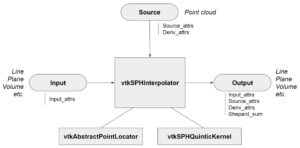
There are two basic approaches to point interpolation as implemented in the vtkPointInterpolator and vtkSPHInterpolator classes. Both of these classes provide a framework for interpolation using different computational kernels, and both are implemented in multi-threaded form via vtkSMPTools so are quite fast on multi-core computing systems. The basic usage pattern of these filters is depicted in the diagram below. Typically the user supplies an input data set onto which s/he wishes to interpolate data from a source point cloud. A computational kernel is specified (in this example a quintic-order SPH kernel) and a point locator is optionally supplied (by default a vtkStaticPointLocator is used, more on this in a moment). The kernel is invoked repeatedly on multiple threads, and simply interpolates data from nearby points onto each probe point of the input dataset.

Given a probe point, the locator plays the critical role of identifying nearby points (which is computationally expensive) and must be chosen and configured properly for maximum performance. As mentioned, a vtkStaticPointLocator is used by default, which is a threaded, uniform binning locator that is very fast in most applications. However, in some situations with extreme variation in point density, other hierarchical locators such as KD-tree (vtkKdTreePointLocator) and octree (vtkOctreePointLocator) may perform better.

The meat of the algorithm can be found in the kernels. The vtkSPHInterpolator uses kernels of subclass vtkSPHKernel; while the vtkPointInterpolator uses kernels of type vtkGeneralizedKernel. These types of interpolation vary in that the SPH process corresponds to physical processes and require a density array, with an optional mass array and cutoff distance array possible. (The cutoff distance specifies a sphere in which the local probe neighborhood is defined.) On the other hand, the vtkPointInterpolator supports a variety of general kernels including

• Linear — average the values of the neighborhood points
• Voroni — interpolate from the closest point
• Shepard — use a Shepard weighting function (the exponent order can be defined)
• Gaussian — use a weighted Gaussian function
• Elliptical Gaussian — a Gaussian function weighted in the direction of the normal

The kernels have methods to define the local neighborhood. In the SPH formulation, a cutoff radius is defined. vtkGeneralizedKernels neighborhoods may be defined as all points within a radius, or as the N closest points.

A variety of SPH kernels are defined as well. These are spline formulations ranging from cubic to quintic, with new kernels in the process of being added (e.g., the Wendland 5th order kernel was contributed to VTK in September). See this reference [11] for the details of the SPH interpolation formulation.

In VTK using Python, the use of these kernels is demonstrated below. For a SPH kernel using the default locator:

  sphKernel = vtk.vtkSPHQuinticKernel()
  sphKernel.SetSpatialStep(0.1)

  interpolator = vtk.vtkSPHInterpolator()
  interpolator.SetInputConnection(plane.GetOutputPort())
  interpolator.SetSourceConnection(input.GetOutputPort())
  interpolator.SetKernel(sphKernel)
  interpolator.Update()

Similarly for generalized interpolation manually specifying a locator and an input point cloud:

  locator = vtk.vtkStaticPointLocator()
  locator.SetDataSet(output)
  locator.BuildLocator()

  gaussianKernel = vtk.vtkGaussianKernel()
  gaussianKernel.SetSharpness(4)
  gaussianKernel.SetRadius(0.5)

  interpolator = vtk.vtkPointInterpolator()
  interpolator.SetInputConnection(plane.GetOutputPort())
  interpolator.SetSourceData(output)
  interpolator.SetKernel(gaussianKernel)
  interpolator.SetLocator(locator)
  interpolator.SetNullPointsStrategyToNullValue()

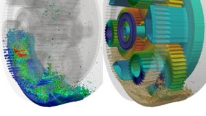
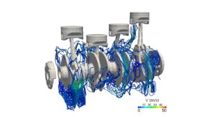
The figures below, courtesy of Altar Engineering / FluiDyna GmbH (who by the way supported much of this work) are examples of SPH interpolation in computational fluid dynamics. Typically the approach is to simulate complex flow on high-performance computing systems, and then resample the results onto a 3D volume, plane or line probe to better visualize the results.

Making It Easy With ParaView

Of course developing an application with VTK takes work and this is where ParaView comes in. As most of you know, ParaView is a premiere visualization application built on VTK developed for large-scale computing challenges. And the good news here is that point interpolation has been added to ParaView with the recent 5.1 release. In ParaView, it is possible to use interactive widgets to define volumes, planes, and polylines to resample point clouds and rapidly display them using volume rendering or other standard visualization techniques. These topics are covered in the next article in this series.

References

1. https://en.wikipedia.org/wiki/Project_Tango
2. https://en.wikipedia.org/wiki/Kinect
3. https://en.wikipedia.org/wiki/Smoothed-particle_hydrodynamics#Uses_in_fluid_simulation
4. https://blog.kitware.com/rendering-engine-improvements-in-vtk/
5. https://blog.kitware.com/volume-rendering-improvements-in-vtk/
6. https://blog.kitware.com/new-opengl-rendering-in-vtk/
7. http://www.vtk.org/Wiki/VTK/Remote_Modules
8. https://gitlab.kitware.com/ken-martin/vtkLODPointCloudMapper
9. https://gitlab.kitware.com/vtk/point-cloud.git
10. https://blog.kitware.com/simple-parallel-computing-with-vtksmptools/
11. D.J. Price, Smoothed particle hydrodynamics and magnetohydrodynamics, J. Comput. Phys. 231:759-794, 2012. Especially  equation 49.