GeoWATCH
GeoWATCH is a powerful tool designed to train, predict, and evaluate AI models on complex heterogeneous sequences of imagery. While initial development focused on geospatial satellite imagery, it is designed for any sequence of rasters. Unlike traditional tools, it’s built to handle diverse sensor data, accommodating variations in band type, resolution, and revisit rates. This flexibility empowers GeoWATCH to provide valuable insights across domains, from satellite imagery analysis to effectively any problem that requires jointly considering sequences of raster data.
The GeoWATCH code is open source and available on PyPI, with documentation, tutorials, source code, and resources accessible at the end of this article
Key Features: What Sets GeoWATCH Apart?
We designed GeoWATCH to train neural networks that could consider all available information from whatever sensors happen to be available or applicable to a problem. Here are a few ways GeoWATCH stands out:
- Adaptive Data Sampling
- Leveraging an “in-situ” data sampling approach, GeoWATCH’s data loaders only retrieve data necessary for training. It provides a “virtual grid system” that avoids the need for extensive duplication and reduces storage demands, ensuring efficient data access and processing.
- Fine-Grained Control Over Parameters
- Users can configure parameters like window resolution, input resolution, and temporal sampling to fine-tune the data according to the specific requirements of a task.
- Rich Dataloader Features
- GeoWATCH supports advanced data loading options like class balancing, normalization, and other preprocessing methods that simplify the pipeline while ensuring a high-quality dataset for model training.
- Intuitive COCO-Like Structure
- With COCO-style inputs and outputs (using our KWCoco library), GeoWATCH remains user-friendly and integrates seamlessly into familiar machine learning workflows.
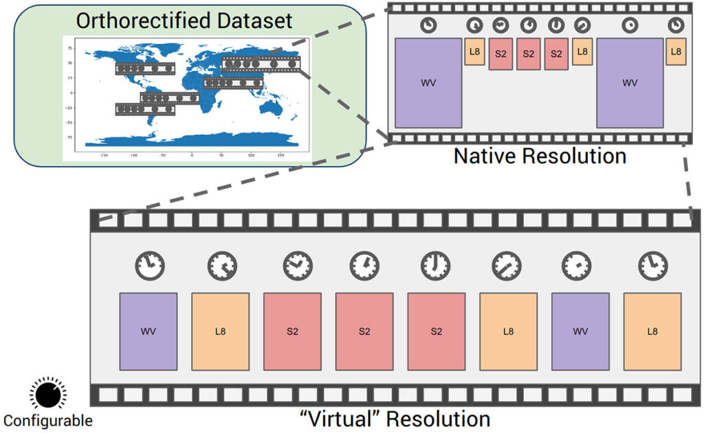
To illustrate the data flexibility provided by GeoWATCH consider the geospatial problem of detecting objects (e.g. buildings, farmland, sea ice) or events (e.g. construction, animal migrations, oil spills) from different sensors orbiting the earth, each with different bands, resolutions, revisit rates, and different costs of acquiring data. Each area of interest on the earth may have a different set of images that provide observations at different times. A naive approach may be to resample all data to the same resolution on disk and only take sets of comparable spectral bands. However, this is undesirable because it requires extra disk space to store the processed data, and if the resampling strategy changes, the preprocessing pipeline needs to be rerun. Instead, we opt to build a system that “virtually resamples” this data for conceptual clarity, but at sample time, any set of resolutions or bands can be accessed. This includes sequences of images at their native resolution (e.g. this means a 30m GSD Landsat-8 image might be 100×100 pixels and a 10m GSD Sentinel-2 image would be 300×300 pixels, but the 4 corner pixels in each image would be aligned). This virtual resampling is illustrated in Figure 1.
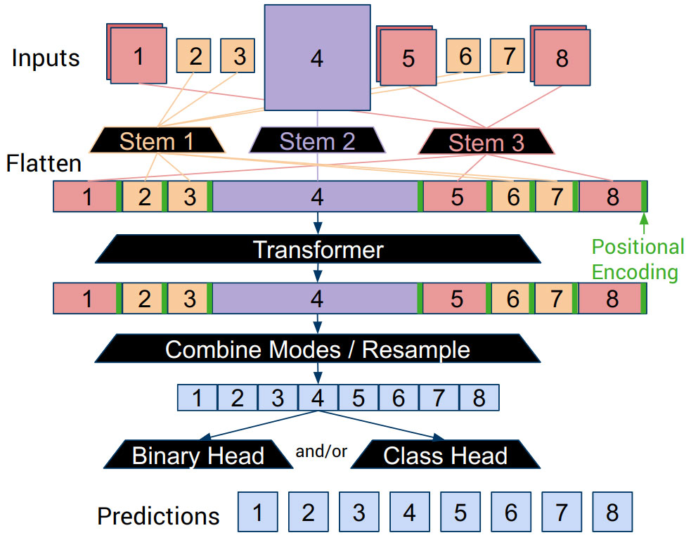
Given a sequence of sampled imagery, the question becomes: what do we do with it? We pass it through a neural network, of course! There are several ways this can be done, but we currently opt to have a per-sensor “stem” to adapt potentially different numbers of bands from each sensor into a compatible “tokenizable” format. From there, we can pass the sequences of tokens through a transformer network, which can have any number of heads attached to it for different tasks.
Current Applications
GeoWATCH has been applied in a wide array of real-world problems, underscoring its versatility and robustness. Here we highlight several of them.
Heavy Construction Event Detection
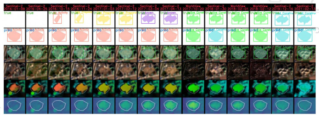
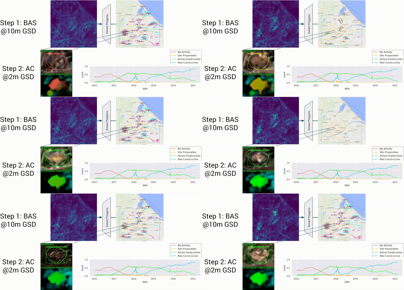
The heavy construction task requires the most complex set of inputs and outputs. This also happens to be the use case that motivated the system design. Specifically, we were motivated to build a system that could ingest Landsat-8, Sentinel-2, Worldview, and PlanetScope imagery as part of the IARPA SMART challenge. One of the construction sites that we detected and characterized as part of this challenge is illustrated in Figure 3. This shows a sequence of images (simplified for visualization) and compares the GeoWATCH predictions to truth labels.
For the heavy construction task, we utilize two networks. The first is a low-resolution detection network that highlights areas to investigate further, and the second is that zooms in on a detected area and makes a final decision about what activity is occurring. This two-stage system is illustrated in Figure 4. For this heavy construction application, we have also built a web-based application called RDWATCH that allows for further visualization and exploration of these results.
Disaster Response and Building Damage Assessment
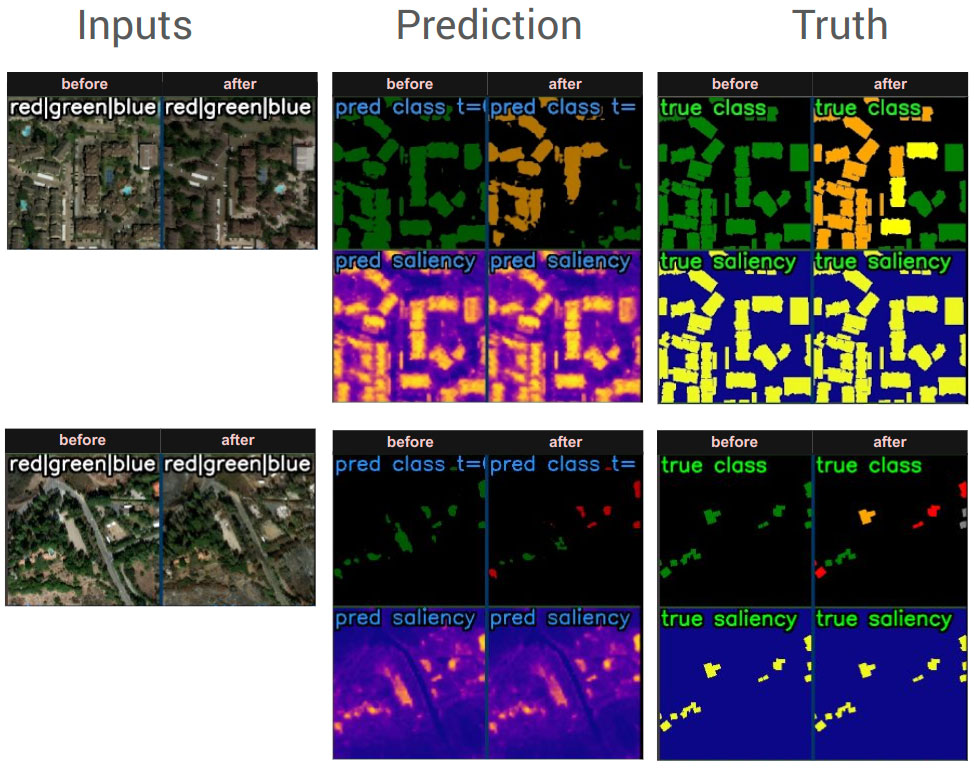
Moving to a simpler example, consider the xView2 building damage assessment. In this case, only two images from the same sensor are given as input, and the task is to detect buildings and classify the severity of damage. Example predictions on this problem are illustrated in Figure 5.

Honey Bee Tracking
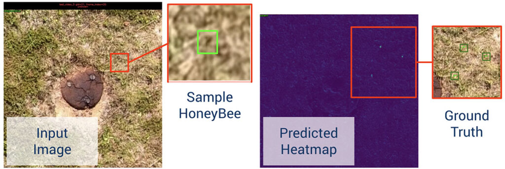
We have also used GeoWATCH to detect and track small objects in video sequences: specifically, we have tracked the movement of honey bees in video data. Due to the resolution of the video, the bees are small and nearly impossible to see in a single frame. However, because GeoWATCH can reason and predict over multiple frames, the system can find the bees as they fly around the scene. A honey bee tracking result is illustrated in Figure 6.
Dog Poop Detection
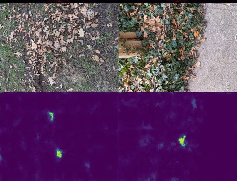
On the other end of the task complexity spectrum, GeoWATCH’s dataloader and networks can handle loading and predicting heatmaps on simple single-image RGB rasters. One example is this author’s pet project: “ScatSpotter,” which has the goal of helping dog owners use the camera on their smartphone to detect their pet’s feces in cluttered environments. A set of promising preliminary results is illustrated in Figure 7.
Algal Bloom Detection & Severity Classification
We applied GeoWATCH to the TickTickBloom challenge. This challenge used sequences of Landsat-8 and Sentinel-2 images to classify if a harmful algal bloom was occurring and its severity. Despite only dedicating effort to collecting data, our system scored reasonably well and above the baseline with little tuning.
Standard Machine Learning Classification Benchmarks
We have applied geowatch to study simple classification problems on datasets like CIFAR-10 and Functional Map of the World. In these cases, the images are fixed-sized on a disk with a classification label. We aim to make the GeoWATCH system useful in both production and research environments.
Future Potential
GeoWATCH is positioned for growth, capable of expanding to any task in semantic segmentation—or more generally, any task where the desired output is a probability raster. Here’s what’s next:
- New Model Integrations
- GeoWATCH will incorporate state-of-the-art techniques like self-supervised learning (e.g., ScaleMAE) for data-efficient model training and high-performance computing (HPC) scalability. We also plan to incorporate pre-trained vision language models (VLMs) to build on the investment the AI community has made in training foundational models.
- Flexible Deployment
- Designed for low-SWAP (Size, Weight, and Power) deployment, GeoWATCH is suitable for building models that can be deployed in constrained environments, from edge devices to field-deployed systems. We have been able to convert our models into TensorRT, which provides high-performance inference.
- Sensor Versatility
- GeoWATCH supports data from various sensors with arbitrary bands. We plan to experiment with more sensor types, including Synthetic Aperture Radar (SAR) and Synthetic Aperture Sonar (SAS). These sensors provide reliable information even under challenging conditions, such as low light or adverse weather, broadening GeoWATCH’s applications to include maritime surveillance, environmental monitoring, and disaster assessment.
- Exploratory “What-If” Analyses
- GeoWATCH can support predictive analyses, exploring potential future states based on historical trends, a valuable tool in agriculture, commercial insurance, environmental monitoring, and beyond. Technically, this can be done using transformer decoders and positional encodings to represent user queries.
With these future capabilities, GeoWATCH aims to be a practical tool for complex image analysis, designed to handle diverse data sources and adaptable to various field and lab settings.
For more details about our future plans, see our roadmap documentation. GeoWATCH is an open source package that is available on PyPI and developed on Gitlab (contributions welcome!). Included in the code are several tutorials that can be used to build your own model or use one of our publicly available models. We recommend starting with Tutorial #1, where we demonstrate how to build a simple RGB model on toy data. API-level documentation is available on ReadTheDocs. We have also published several academic papers using GeoWATCH, which can be found here:
Interested in leveraging GeoWATCH’s capabilities for your project or looking for more details? Contact us, and we would be glad to help!
Like this article? Also check out our article on RDWATCH, an advanced cloud-ready system designed to streamline machine learning workflows for monitoring, annotating, and visualizing geospatial and georeferenced data.
Acknowledgment
This research is based upon work supported in part by the Office of the Director of National Intelligence (ODNI), Intelligence Advanced Research Projects Activity (IARPA), via 2021-201100005. The views and conclusions contained herein are those of the authors and should not be interpreted as necessarily representing the official policies, either expressed or implied, of ODNI, IARPA, or the U.S. Government. The U.S. Government is authorized to reproduce and distribute reprints for governmental purposes, notwithstanding any copyright annotation therein.