Bivariate Representations in ParaView

September 10, 2024

In the context of scientific visualization, simulation outputs may contain various scalar fields. Studying multiple fields simultaneously as well as their correlations may be of interest to analysts. It then becomes a necessary issue for ParaView to offer adequate visualization tools allowing multivariate rendering.

In this blog post, we will present several tools recently introduced in ParaView dedicated to bivariate rendering. We introduced volume bivariate visualization and analysis abilities in ParaView starting from version 5.11.0. Here, we give a special focus on a new plugin available since ParaView 5.12.0, bringing several new bivariate representations for surfaces.

Volumic bivariate visualization

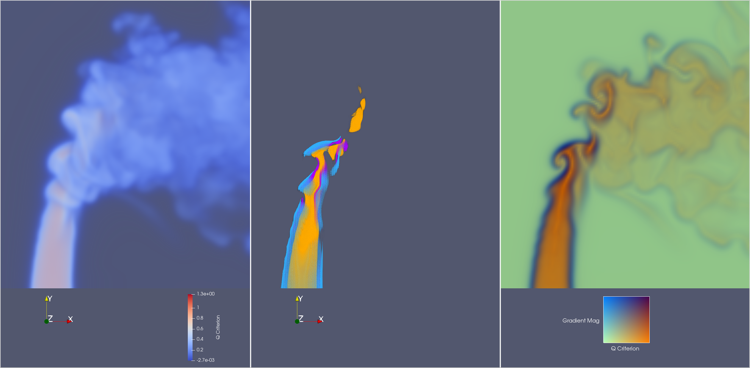
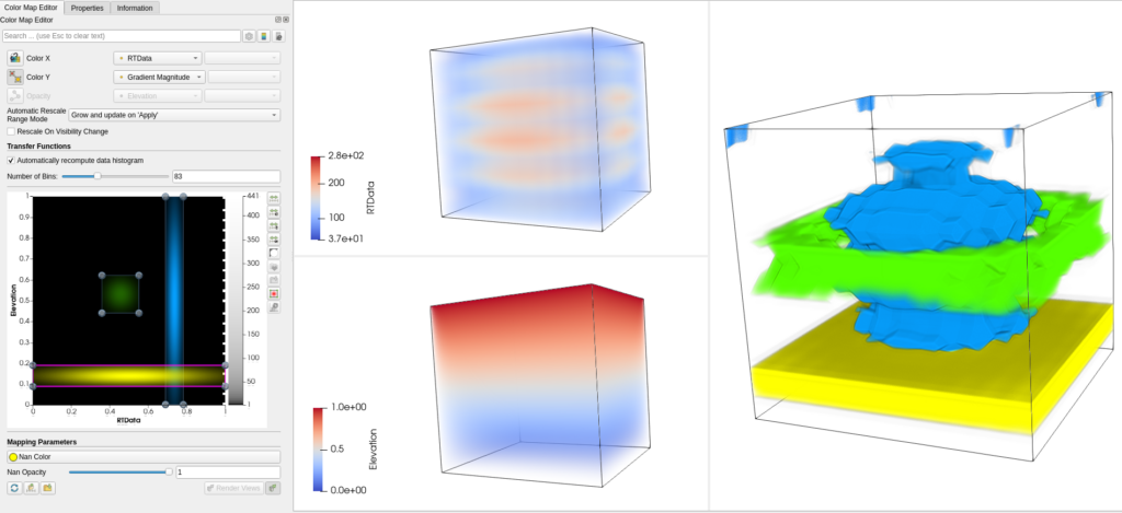
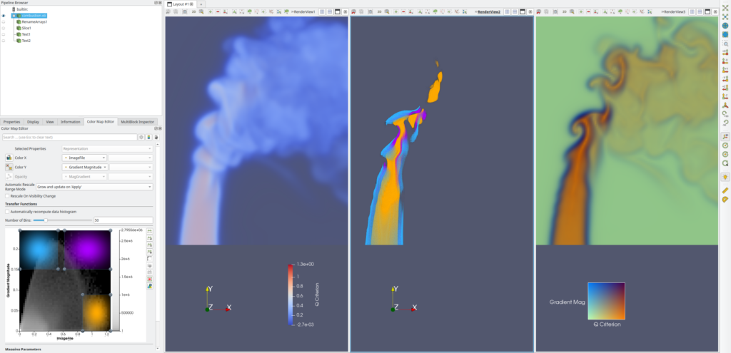
Since ParaView 5.11.0, bivariate visualization has been possible when using the `Volume` representation (thus limited to regular rectilinear grids). For this purpose, the “GPUVolumeMapper” can use 2D transfer functions to use combined information to disambiguate areas that fall within a given range for 2 parameters simultaneously. Thanks to a dedicated scatter plot widget, you can control 2D gaussian curves that drive the visible parts of the data (cf, image below with the green, blue and yellow area). Note that gradient magnitude values of the first selected field are automatically generated and can be used as second field, allowing the visualization of big changes in values spatially (and highlight features). More information about this feature can be found in this previous blog post.

Example of usage of the 2D transfer function: the scatter plot on the left allows to define “boxes” (color gaussians) to highlighting areas of interest and study the degree of correlation between the 2 variables.

The VTK “GPUVolumeMapper” also makes it possible to use separate transfer functions, one for color and one for opacity with two different arrays, allowing to visualize two fields of data at the same time. This is a simple but sometimes cluttered way to represent two pieces of information at the same time during rendering, because transparency tends to hide information about the colored field.

*Example of volume rendering with coloring done according to elevation, and opacity bound to a wave function*

The “Bivariate Representations” plugin

Available since ParaView 5.12, the “Bivariate Representations” plugin extends bivariate visualization and analysis to surfacic representations, so available for both structured and unstructured data sets. As we will see in the next sections, there are different ways to render two data fields simultaneously on surfaces, involving colors, opacity or even time. Note that these two representations are intrinsically limited to point data arrays.

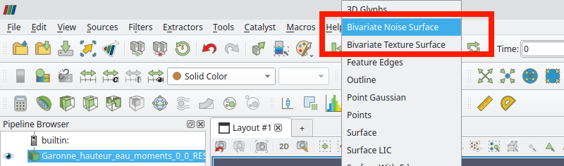
But before going into detail, let’s see how to enable these new representations. The “Bivariate Representations” plugin is now shipped in the binaries of ParaView: to enable it, simply go to Tools -> Load Plugin… and select “BivariateRepresentations”.

*The “Bivariate Representations” plugin in ParaView’s Plugin Manager*

In the current state, the “BivariateRepresentation plugin” adds 2 new representations to render views. These representations are accessible from the representations drop-down menu like any other representation (please note that if you just loaded the plugin, creating a new render view is necessary to refresh the available representations).

*The two bivariate representations are added to the drop-down menu*

Bivariate Texture Representation

The first representation is called the “Bivariate Texture Representation”. It corresponds to a classical approach to visualize surfacic bivariate data, by using a 2D color map to assign color to values provided by 2 different arrays. Note that for now, this representation is limited to vtkPolyData, so you may use of the “Extract Surface” filter on your data beforehand.

This representation makes use of the existing ParaView mechanism for applying 2D textures on surfacic geometry representations. Under the hood, the “Bivariate Texture Representation” simply computes texture coordinates from the first and second array, mapping their values to coordinates between 0 and 1 in X and Y direction respectively. The 2 arrays should be selected through a dedicated section; the array color should stay to “Solid Color” to not interfere with texture coloring.

The generated 2D array containing texture coordinates is recomputed each time the 2 input arrays change, and is added to the list of available texture arrays as “BivariateTCoords”. These arrays are accessible through the “Texture Coordinate” display properties.

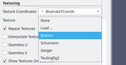
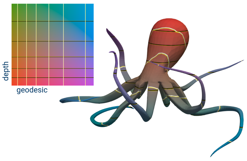
*Four default 2D textures available in the Bivariate Texture Representation.* *Credits: Steiger & Al. [3] [4]*

Once the 2D array is selected, we can choose the texture to apply. The “Bivariate Texture Representation” comes along with four 2D color textures suitable for bivariate analysis, originating from the work of Steiger & Al. [3] [4]. It’s also possible to upload and use custom textures to highlight a specific correlation between the fields or different sets of levels (isocontours), as shown in the image below.

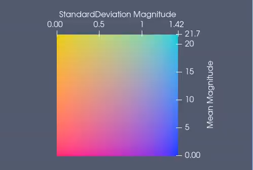
*Usage of a custom texture (constant color around X = Y) to produce fibers*. *Data: 2D von Karman vortex street [5]*

*Usage of a custom texture on an octopus 3D model [7] to create isocontours.*

Once selected, a representation of the texture will be visible in the render view to act as a legend.

Note that the Bivariate Texture Representation supports texture with opacity. Such textures can be used to highlight zones of interest, echoing the usage of color gaussians in the volume presentation discussed earlier.

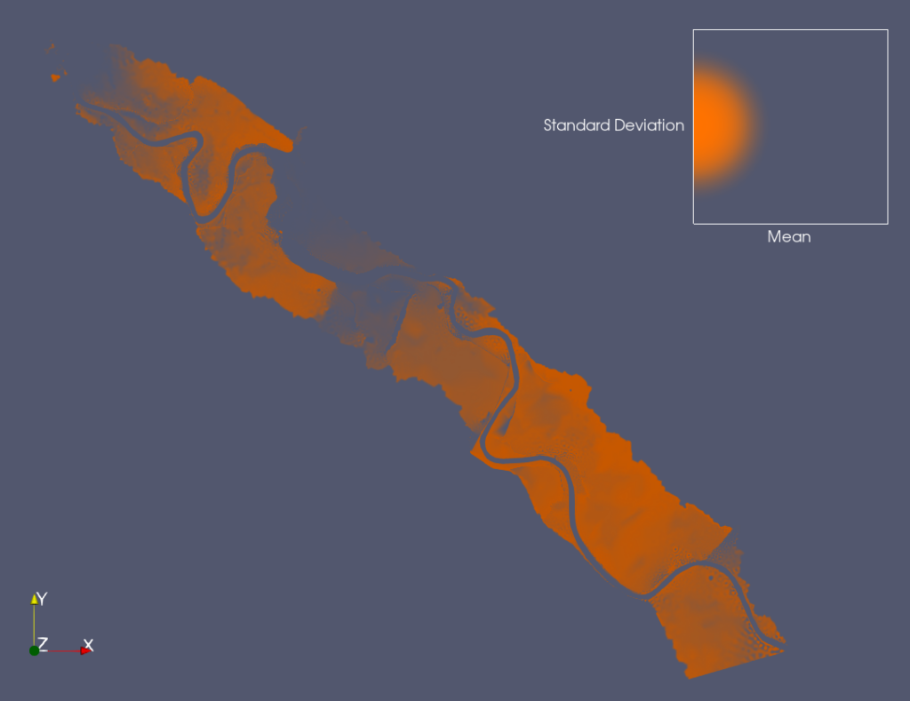
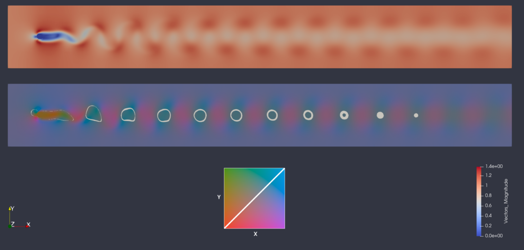
*“Bivariate Texture Representation” with opacity*. *Dataset: Study case of the Garonne River [1] [2]*

Bivariate Noise Representation

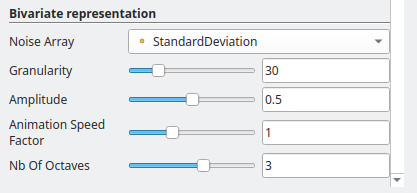
The second bivariate representation is called “Bivariate Noise Representation”. It relies on dynamic Perlin noise, varying through time, to alter the color given by the “Coloring Array” (first data field) depending on the values of the “Noise Array” (second data field). For a given point on the surface, the higher the values of the “Noise Array,” the greater the intensity of the color oscillation.

This representation exposes four parameters that can be used to control the generation of the Perlin noise:

Granularity: the frequency of the noise, i.e. it’s spatial definition;
Amplitude: the amplitude of the noise, i.e. how strongly the values of the second array alter the color of the first one;
Animation speed factor: factor modifying the speed animation of the noise oscillations
Nb of octaves: number of overlapping layers of noise, controlling the “sharpness” of the final result (can noticeably impact performance)

*Bivariate Noise Representation display parameters*

If this representation does not allow very precise bivariate analysis, its dynamic factor makes it great for presentations. We illustrate it in the example below, which represents a typical usage of bivariate representation: display a field of scalar value and its measurement uncertainty.

Conclusion & further improvements

The support of bivariate rendering in ParaView brings new prospects for data analysis. These features are beneficial to both surfacic and volumic datasets and can greatly facilitate the study of simultaneity, correlation or uncertainty of the observed data fields.

Comparison of 3 rendering modes: Q-criterion vs it’s gradient magnitude. On the left, volume rendering of the Q-criterion alone. On the middle, we use volume rendering with the 2D transfert function to highlight specific values of both fields. On the right, we display a slice with the “Bivariate Texture Representation” to have a global overview of the two fields. *Dataset: “Q-criterion of a jet in crossflow created by a direct numerical simulation.” [6]*

Future efforts will focus on an overall polishing of the “Bivariate Texture Representation” in terms of features and user experience. First and foremost, these improvements would be:

allowing the “Bivariate Texture Representation” to support any surfacic representation without polydata conversion,
implementing a dedicated and editable 2D scalar bar in the render view, with axes and legend,
reducing the number of user interactions required to set up the texture coordinates,
and in general, unifying both bivariate representation properties in the UI.

*Example of 2D “Scalar Bar” in ParaView*

We will keep you informed about the development of these new features, so stay tuned for future posts!

Acknowledgement

This work was supported by EDF

[1] Besnard, A., & Goutal, N. (2011). Comparaison de modèles 1D à casiers et 2D pour la modélisation hydraulique d’une plaine d’inondation – Cas de la Garonne entre Tonneins et La Réole. La Houille Blanche, 97(3), 42–47. https://doi.org/10.1051/lhb/2011031

[2] Goeury, Cédric & David, T & Ata, Riadh & Audouin, Yoann & Goutal, Nicole & Popelin, A.-L & Couplet, M & Baudin, Michaël & Barate, R. (2015). UNCERTAINTY QUANTIFICATION ON A REAL CASE WITH TELEMAC-2D.

[3] Steiger, M., Bernard, J., Thum, S., Mittelstädt, S., Hutter, M., Keim, D.A., & Kohlhammer, J. (2015). Explorative Analysis of 2 D Color Maps.

[4] https://github.com/dominikjaeckle/Color2D

[5] http://gerris.dalembert.upmc.fr/examples

[6] Grout, R. W., Gruber, A., Kolla, H., Bremer, P.-T., Bennett, J. C., Gyulassy, A., & Chen, J. H. (2012). A direct numerical simulation study of turbulence and flame structure in transverse jets analysed in jet-trajectory based coordinates. Journal of Fluid Mechanics, 706, 351–383. doi:10.1017/jfm.2012.257

[7] Octopus 3D model from https://www.3dcadbrowser.com/3d-model/octopus